Training, Tracking, Analyzing, Interpreting and Serving Models with One Line of Code

As a data scientist, rapid experimentation is extremely important. If an idea doesn’t work it’s best to fail quickly and find out sooner rather than later.

When it comes to modelling, rapid experimentation is already fairly simple. All model implementations follow the same API interface so all you have to do is initialize the model and train it. The problem comes now when you have to interpret, track, and compare each model.

Do you make a large notebook with all your models and scroll up and down or use a table of contents to see the results of different models? Do you create a different notebook for each model and then flip back and forth between notebooks? How do you track iterations of the models if you start tweaking the parameters? Where do you store artifacts to revisit at a later date or for further analysis?

I’m going to demonstrate a way to address these problems by training multiple models, each with 1 line of code, view the overall results easily, analyze the models, interpret the models, track the models in MLFlow and serve them using Aethos.

Prepping the Data

We’ll use Aethos to quickly prep the data. For more information on how to analyze and transform your datasets with Aethos, check out my previous blog post here. Load the Titanic training data from the Aethos repo.

import aethos as at  
import pandas as pd

data = pd.read_csv('https://raw.githubusercontent.com/Ashton-Sidhu/aethos/develop/examples/data/train.csv')

Pass the data into Aethos.

df = at.Data(data, target_field='Survived')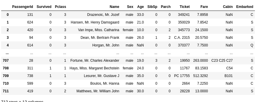

The focus of this post is modelling so let’s quickly preprocess the data. We’re going to use the Survived, Pclass, Sex, Age, Fare and Embarked features. insert here

df.drop(keep=['Survived', 'Pclass', 'Sex', 'Age', 'Fare', 'Embarked'])
df.standardize_column_names()

Replace the missing values in the Age and the Embarked columns.

df.replace_missing_median('age')  
df.replace_missing_mostcommon('embarked')

Normalize the values in the Age and Fare columns and One Hot Encode the Sex, Pclass and Embarked features.

df.onehot_encode('sex', 'pclass', 'embarked', keep_col=False)  
df.normalize_numeric('fare', 'age')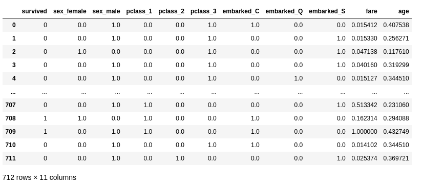

With Aethos, the transformer is fit to the training set and applied to the test set. With just one line of code both your training and test set have been transformed.

Modelling

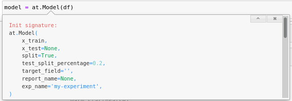
To train Sklearn, XGBoost, LightGBM, etc. models with Aethos, first transition from the data wrangling object to the Model object.

model = at.Model(df)

The model object behaves the same way as the Data object so if you have data that has already been processed, you can initiate the Model object the same way as the Data object.

Next, we’re going to enable experiment tracking with MLFlow.

at.options.track_experiments = True

Now that everything is set up, training a model and getting predictions is as simple as this:

lr = model.LogisticRegression(C=0.1)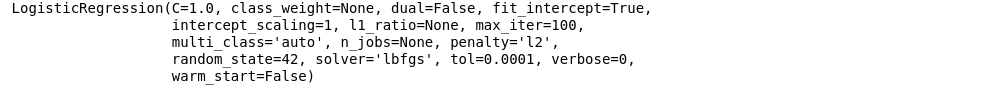

To train a model with the optimal parameters using Gridsearch, specify the gridsearch parameter when initializing the model.

lr = model.LogisticRegression(gridsearch={'C': [0.01, 0.1]}, tol=0.001)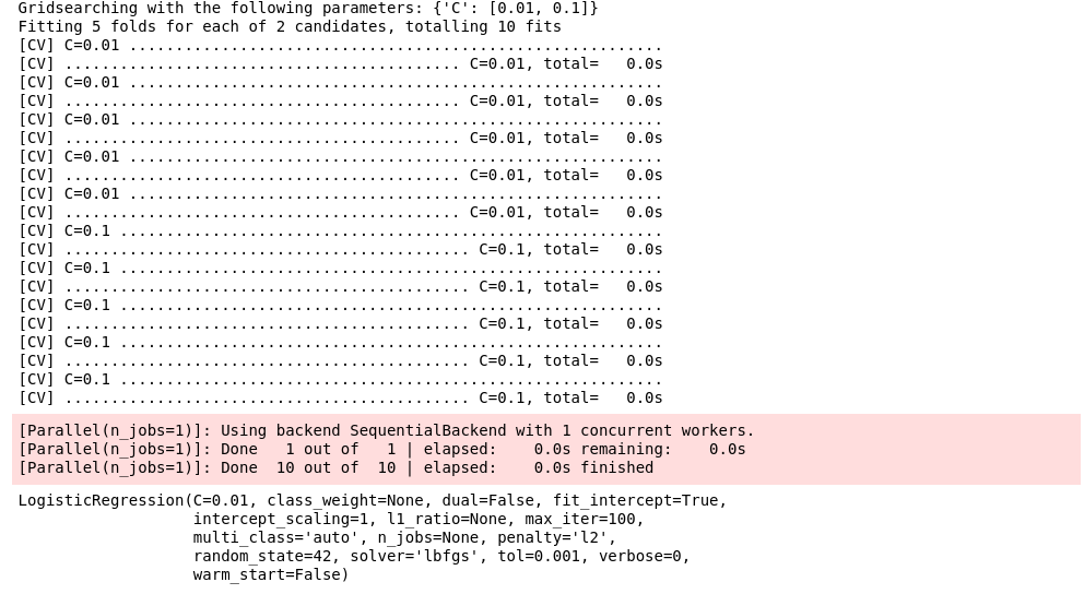

This will return the model with the optimal parameters defined by your Gridsearch scoring method.

Finally, if you want to cross validate your models there are a few options:

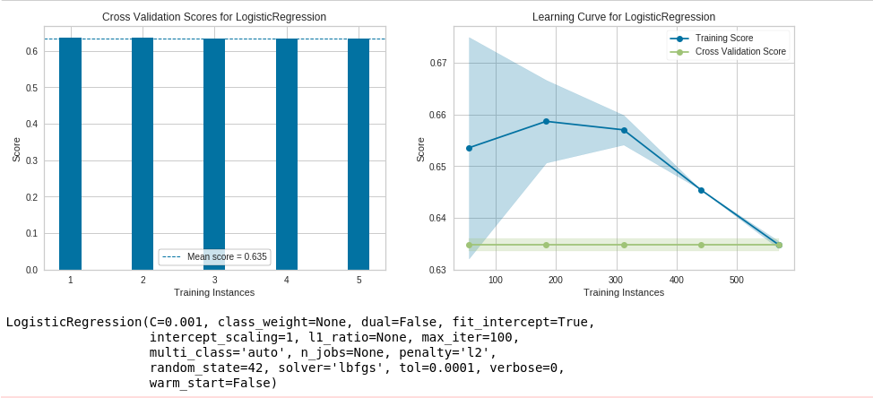
lr = model.LogisticRegression(cv=5, C=0.001)

This will perform 5-fold cross validation on your model and display the mean score as well as the learning curve to help gauge data quality, over-fitting, and under-fitting.

You can also use it with Gridsearch:

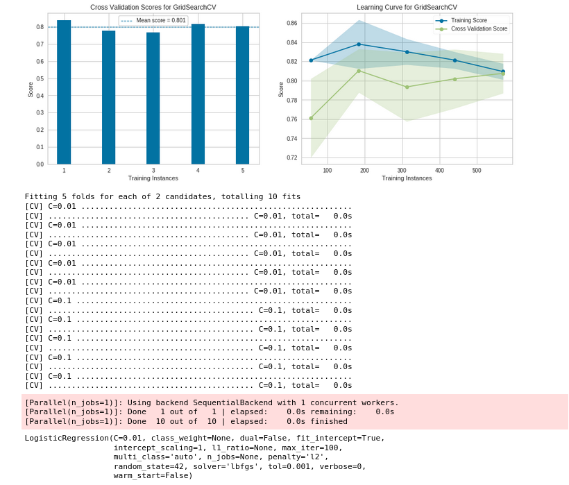
lr = model.LogisticRegression(cv=5, gridsearch={'C': [0.01, 0.1]}, tol=0.001)

This will first use Gridsearch to train a model with the optimal parameters and then cross validate it. Currently supported cross validation methods are k-fold and stratified k-fold.

To train multiple models at once (in series or in parallel) specify the run parameter when defining your model.

lr = model.LogisticRegression(cv=5, gridsearch={'C': [0.01, 0.1]}, tol=0.001, run=False)

Let’s queue up a few more models to train:

model.DecisionTreeClassification(run=False)  
model.RandomForestClassification(run=False)  
model.LightGBMClassification(run=False)

You can view queued and trained models by running the following:

model.list_models()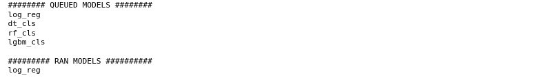

To now run all queued models, by default in parallel:

dt, rf, lgbm = model.run_models()

You can now go grab a coffee or a meal while all your models are trained simultaneously!

Analyzing Models

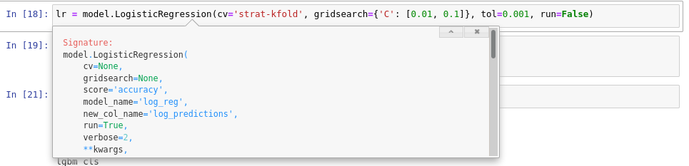
Every model you train by default has a name. This allows you to train multiple versions of the same model with the same model object and API, while still having access to each individual model’s results. You can see each model’s default name in the function header by pressing Shift + Tab in Jupyter Notebook.

You can also change the model name by specifying a name of your choosing when initializing the function.

First, let’s compare all the models we’ve trained against each other:

model.compare_models()

You can see every models’ performance against a wide variety of metrics. In a data science project there are predefined metrics you want to compare models against (if you don’t, you should). You can specify those project metrics through the options.

at.options.project_metrics = ['Accuracy', 'Balanced Accuracy', 'Zero One Loss']

Now when you compare models, you’ll only see the project metrics.

model.compare_models()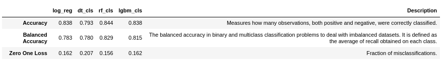

You can also view the metrics just for a single model by running the following:

dt.metrics() # Shows metrics for the Decision Tree model  
rf.metrics() # Shows metrics for the Random Forest model  
lgbm.metrics() # Shows metrics for the LightGBM model

You can use the same API to see each models’ RoC Curve, Confusion matrix, the index of misclassified predictions, etc.

dt.confusion_matrix(output_file='confusion_matrix.png') # Confusion matrix for the Decision Tree model

rf.confusion_matrix(output_file='confusion_matrix.png') # Confusion matrix for the random forest model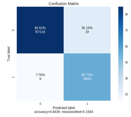

Interpreting Models

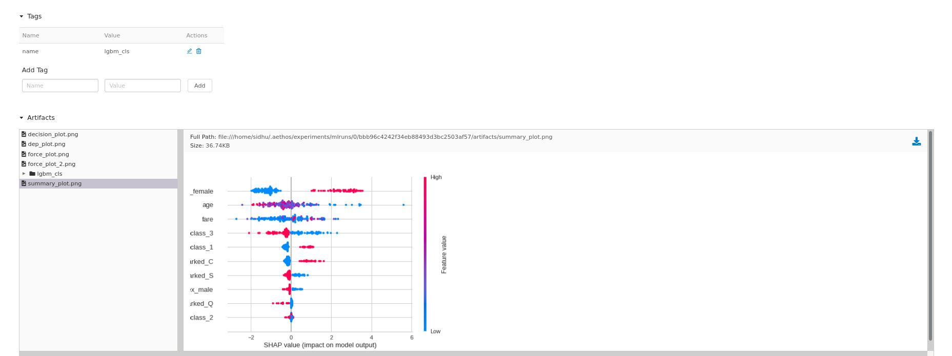
Aethos comes equipped with automated SHAP use cases to interpret each model. You can view the force, decision, summary, and dependence plot for any model — each with customizable parameters to satisfy your use case.

By specifying the output_file parameter, Aethos knows to save and track this artifact for a specific model.

lgbm.decision_plot(output_file='decision_plot.png')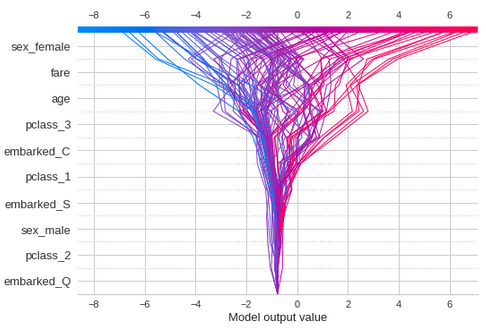

lgbm.force_plot(output_file='force_plot.png')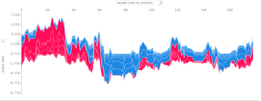

lgbm.shap_get_misclassified_index()  
# [2, 10, 21, 38, 43, 57, 62, 69, 70, 85, 89, 91, 96, 98, 108, 117, 128, 129, 139, 141, 146, 156, 165, 167, 169]  
lgbm.force_plot(2, output_file='force_plot_2.png')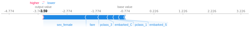

lgbm.summary_plot(output_file='summary_plot.png')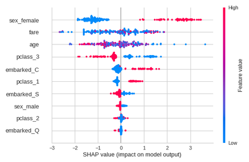

lgbm.dependence_plot('fare', output_file='dep_plot.png')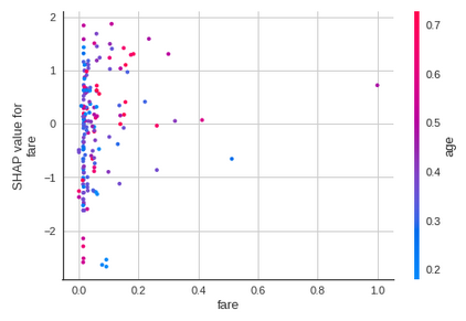

For a more automated experience, run:

lgbm.interpret_model()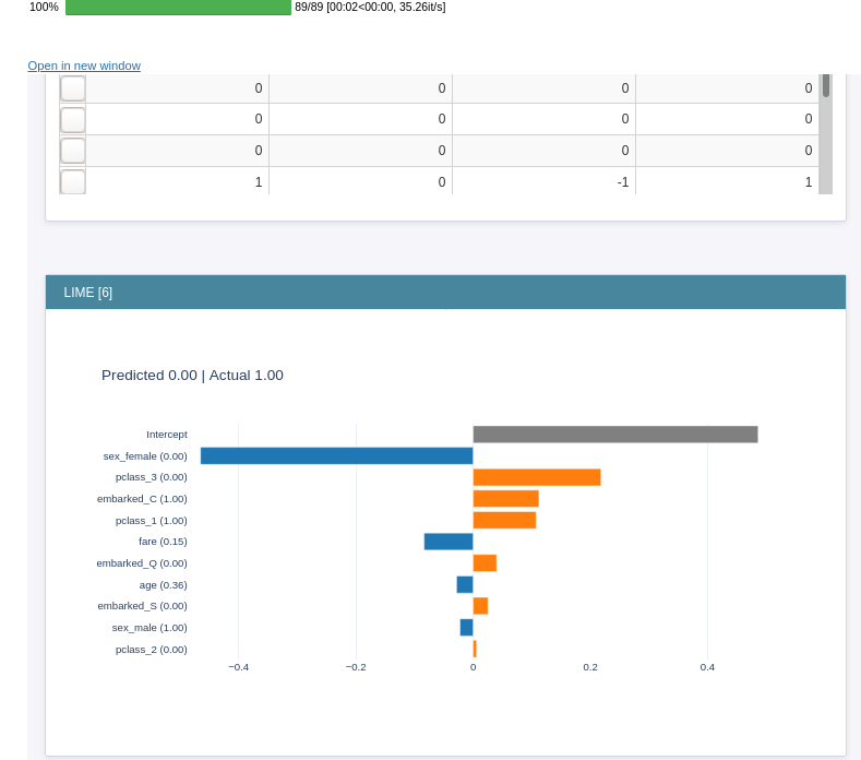

This displays an interactive dashboard where you can interpret your model’s prediction using LIME, SHAP, Morris Sensitivity, etc.

Viewing Models in MLFlow

As we were training models and viewing results, our experiments were automatically being tracked. If you run aethos mlflow-ui from the command line, a local MLFlow instance will be started for you to view the results and artifacts of your experiments. Navigate to localhost:10000.

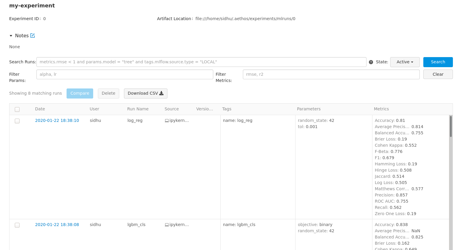
Each of your models and any saved artifacts are tracked and can be viewed from the UI, including parameters and metrics! To view and download model artifacts, including the pickle file for a specific model, click on the hyperlink in the date column.

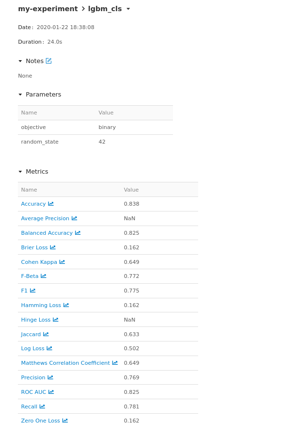
You get a detailed breakdown of the metrics for the model as well as the model parameters and towards the bottom, you will see all your saved artifacts for a specific model.

Note: Cross validation learning curves and mean score plots are always saved as artifacts.

To change the name of the experiment ( by default it is my-experiment) specify the name when initiating the Model object ( exp_name), otherwise every model will get added to my-experiment.

Serving Models

Once you’ve decided on a model you want to serve for predictions, you can easily generate the required files to serve the model with a RESTful API using FastAPI and Gunicorn.

dt.to_service('titanic')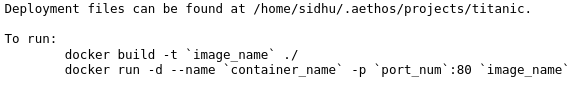

If you’re familiar with MLFlow, you can always use it to serve your models as well. Open a terminal where the deployment files are being kept. I recommend moving these files to a git repository to version control both the model and served files.

Follow the instructions to build the docker container and then run it detached.

docker build -t titanic:1.0.0 ./  
docker run -d --name titanic -p 1234:80 titanic:1.0.0

Now navigate to localhost:1234/docs to test your API. You can now serve predictions by sending POST requests to 127.0.0.1:1234/predict.

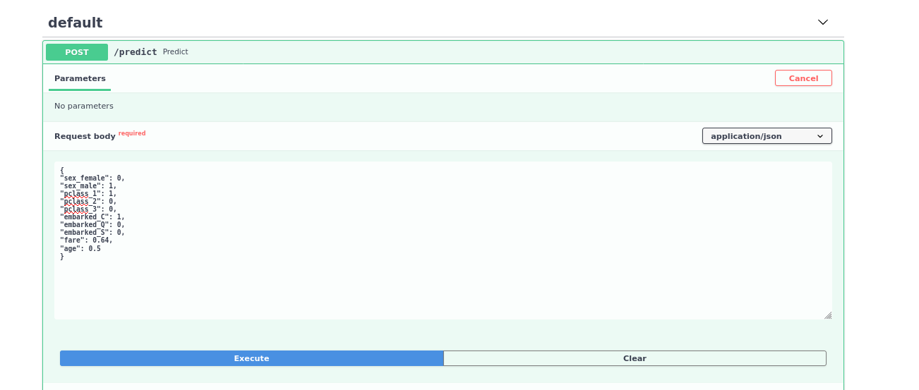
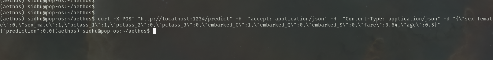
Now one big thing to note, this is running a default configuration and should not be used in production without securing it and configuring the server for production use. In the future, I will add these configurations myself so you can more or less “throw” a model straight into production with minimal configuration changes.

This feature is still in its infancy and one that I will actively continue to develop and improve.

What Else Can You Do?

While this post is a semi- comprehensive guide of modelling with Aethos, you can also run statistical tests such as T-Test, Anovas, use pretrained models such as BERT and XLNet for sentiment analysis and question answering, perform extractive summarization with TextRank, train a gensim LDA model, as well as clustering, anomaly detection and regression models.

The full example can be seen here!

Feedback

I encourage all feedback about this post or Aethos. You can message me on twitter or e-mail me at sidhuashton@gmail.com.

Any bug or feature requests, please create an issue on the Github repo. I welcome all feature requests and any contributions. This project is a great starter if you’re looking to contribute to an open source project — you can always message me if you need assistance getting started.